EONS v2.0 - Tutorial 2: create and run a 7-states AMPA receptor channel model

Introduction / Purpose:

1. Action: Load E.O.N.S.. To do so, please refer to the load model section of the user manual.
   Consequence:Once you have completed this section, you should be presented with the main interface of EONS, containing an empty model: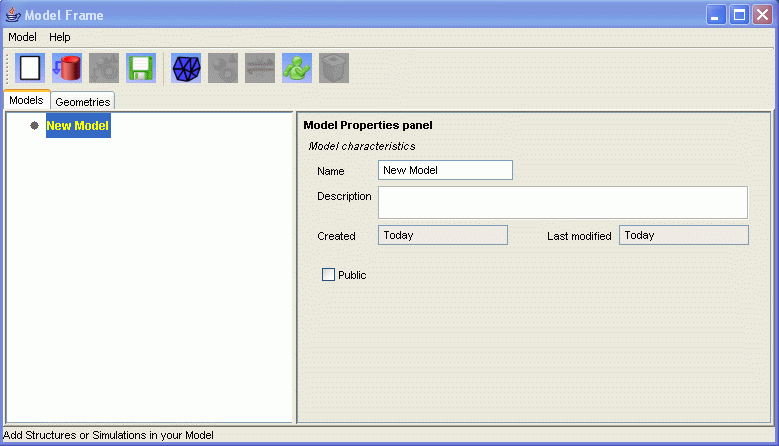


2. Action:Click on the 'Add Structure' button
   Consequence:A new entry appears in the organization tree of your current model. This entry is a structure named 'Structure1' which contains one default element named 'Medium'. Medium is the element selected by default in the organization tree. The right hand side of the interface now displays the properties of the 'Medium' element.


3. Action:Change the name of the 'Medium' element to 'AMPA7states'. The name can be changed either from the organization tree, or from the properties panel. You can also enter a description for this model.
   Consequence:You now have a new element in your current model named 'AMPA7states'.
   
   
   
4. Action: We are now going to add parameters and variables to the AMPA7states element (see the models list page of the reference guide for details on this kinetic model).
   In the properties panel of the 'AMPA7states' element, add the kinetic constants:

   k1 = 8.04 ms-1 . mM-1
   km1 = 1.82 ms-1
   k2 = 4.02 ms-1 . mM-1
   km2 = 3.64 ms-1
   k3 = 0.9 ms-1
   km3 = 0.13 ms-1
   k4 = 0.16 ms-1
   km4 = 0.02 ms-1
   k5 = 0.16 ms-1
   km5 = 0.02 ms-1
   k6 = 0.23 ms-1
   km6 = 0.03 ms-1
   k7 = 3.52 ms-1 . mM-1
   km7 = 3.19 ms-1
   k8 = 1.01 ms-1
   km8 = 0.15 ms-1
   

   In the same way, add the parameters associated with each receptor state (as constants for their initial value and as variables since their value changes during the simulation:

   constant: R = 1
   constant: RL1 = 0
   constant: RdL1 = 0
   constant: RL1L2 = 0
   constant: RdL1L2 = 0
   constant: OL1L2 = 0
   constant: OdL1L2 = 0
   
   variable: R 
   variable: RL1 
   variable: RdL1
   variable: RL1L2
   variable: RdL1L2
   variable: OL1L2 
   variable: OdL1L2 
   

   
   Add the derivatives for each state:

   variable: dR 
   variable: dRL1 
   variable: dRdL1
   variable: dRL1L2
   variable: dRdL1L2
   variable: dOL1L2 
   variable: dOdL1L2 
   

   Add 2 variables to describe the concentration of ligands L1 and L2:

   variable: L1 
   variable: L2 
   

   While adding these parameters to the list, you can also enter a description in their associated Description field.
   Sequencially click on the 'Add to list' button to add all these new constants amd variables to the list of variables for this element.
   
   Consequence:You now have a list of kinetic constants / kinetic states variables defined in the 'AMPA7states' element. Once you have done this, the properties panel of 'MyFirstElement' should display:
   
   


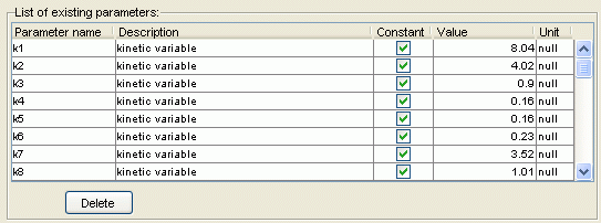
5. Action: Add a new reaction to the 'AMPA7states' element. To do this, make sure that 'AMPA7states' is selected in the model organization tree and click the 'Add reaction' button .
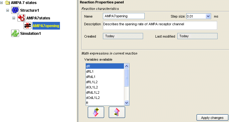
   This will enable you to define the mathematical expressions to be associated with the variables you just created. Let's name this reaction 'AMPA7opening'.
   
   Consequence:You now have a new reaction defined under 'AMPA7states' in the model organization tree. The properties panel of this new reaction named 'AMPA7opening' should display the list of newly created variables:
   
   



6. Action: Assign a mathematical expression to all the variables.
   Select each variable from the list of variables available and click on the 'Add to list' arrow button
   Double click on the 'Mathematical Expression' column corresponding to each variable and enter their corresponding expression
   For each variable, once the mathematical expression has been entered, click on the Enter key of your keyboard.

        Variable           Mathematical Expression
   
   
         L1                 (Vm+70)/1000
         L2                 (Vm+70)/1000
         dR                 diff(R,0.01, - k1 * L1, km1 * RL1)
         dRL1               diff(RL1,0.01, - km1 - k2 * L2 - k4, k1 * R * L1 + km2 * RL1L2 + km4 * RdL1)
         dRdL1              diff(RdL1,0.01, - km4 - k7 * L2, k4 * RL1 + km7 * RdL1L2)
         dRL1L2             diff(RL1L2,0.01, - km2 - k3 - k5, k2 * RL1 * L2 + km3 * OL1L2 + km5 * RdL1L2)
         dRdL1L2            diff(RdL1L2,0.01, - km5 - km7 - k8, k5 * RL1L2 + k7 * RdL1 * L2 + km8 * OdL1L2)
         dOL1L2             diff(OdL1L2,0.01, - km6 - km8, k6 * OL1L2 + k8 * RdL1L2)
         dOdL1L2            diff(OL1L2,0.01, - km3 - k6, k3 * RL1L2 + km6 * OdL1L2) 
   
         R                  (R+dR)/(R+RL1+RdL1+RL1L2+RdL1L2+OL1L2+OdL1L2)
         RL1                (RL1+dRL1)/(R+RL1+RdL1+RL1L2+RdL1L2+OL1L2+OdL1L2)
         RdL1               (RdL1 + dRdL1)/(R+RL1+RdL1+RL1L2+RdL1L2+OL1L2+OdL1L2)
         RL1L2              (RL1L2 + dRL1L2)/(R+RL1+RdL1+RL1L2+RdL1L2+OL1L2+OdL1L2)
         RdL1L2             (RdL1L2 + dRdL1L2)/(R+RL1+RdL1+RL1L2+RdL1L2+OL1L2+OdL1L2)
         OL1L2              (OL1L2 + dOL1L2)/(R+RL1+RdL1+RL1L2+RdL1L2+OL1L2+OdL1L2)
         OdL1L2             (OdL1L2 + dOdL1L2)/(R+RL1+RdL1+RL1L2+RdL1L2+OL1L2+OdL1L2) 
   

   
   Once all mathematical expressions have been entered, click on the 'Apply Changes' button.
   
   Consequence: You just associated mathematical expressions to all the variables in the 'AMPA7states' reaction.
   These mathematical expressions describe the values that will be associated to the variables at every time step. They in turns describe the behavior of the AMPA 7 states element.
   Note 1: The variables L1 and L2 copy the value of the internal variable Vm, offset it and scale it to obtain a reasonable value for a glutamate concentration (in mM). See here for more details on the value of Vm.
   Note 2: The derivative variables call the diff() function. See in the list of functions available in EONS for more details.
   Note 3: The mathematical expressions associated with the variables corresponding to the 7 states of the receptor are all divided by the sum of the 7 states. This ensures that the sum of the probabilities of the system of being in the 7 states remains equal to 1 throughout the simulation.
7. Action: Create a new simulation.
   Now that the model is entirely defined, it is possible to create a simulation for this model. Select the root model in the organization tree.
   Click on the 'Add Simulation' button
   Change the simulation duration from 20 to 50 milliseconds.
   
   Consequence: You just created a new simulation for your current model.
   The parameters for this simulation are:
   • Duration: 50 milliseconds
   • Step size: 0.01 milliseconds.
   
   
8. Action: Generate a correct input signal to your model in the simulation panel. The input signal corresponds to the depolarization.
   The default depolarization selected in the simulation panel is a single pulse depolarization that lasts 5 milliseconds with a 0 milliVolts depolarization (with the baseline being at -70 milliVolts). This modifies the value of the internal variable 'Vm' throughout the simulation.
   Modify the depolarization voltage from 0mV to 30mV
   Consequence: the value of Vm throughout the simulation will be:
   • From 0 to 2 milliseconds ----> -70 mV
   • From 2 to 7 milliseconds ----> +30 mV
   • From 7 to 20 milliseconds ----> -70 mV
   
   The values of L1 and L2 (concentrations of ligands) throughout the simulation will then be:
   • From 0 to 2 milliseconds ----> 0.0 mM
   • From 2 to 7 milliseconds ----> 0.1 mM
   • From 7 to 20 milliseconds ----> 0.0 mM
   
   
9. Action: Select the variables to record in a simulation.
   In the simulation panel, we need to specify the variables that will be recorded. To record a variable, make sure the checkbox next to the variable's name is checked in the table entitled 'parameters to record'.
   In our case, let's select the variables R, L1 and OL1L2.
   
   Consequence: We specified which variables will be recorded throughout the simulation. The interface should look like: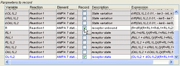
   



10. Action: Verify the parameters that affect the simulation output.
    At the bottom of the simulation panel, you will find a subpanel entitled simulation ouput. This controls the number of points that will be recorded during the simulation. The default selection specifies that 1 point every 10 points is to be recorded for the graphs. Plotting more than 10,000 points results in a significant increase in memory usage, which harms computational speed and does not provide any additional benefit. It is recommended to maintain the number of points between 100 and 5000. In our case, we have a 20 milliseconds simulation and record every 0.01 milliseconds. That constitutes 50/0.01 = 5000 points. Since we only record 1 point every 10, we will plot the graphs with 500 points for each variable. Hence, the default selection is correct and should not be changed.
    
    Consequence: Verification of the number of points recorded at the output.
    



11. Action: Launch the simulation / Display the results.
    Click on the 'Launch simulation' button located at the bottom of the simulation properties panel.
    Consequence: You just launched a new simulation for your current model. During this simulation, the values of all the different variables are calculated. However, only the variables R, L1 and OL1L2 will be recorded. The values of these variables are presented to you in the form of a graph:
    
    



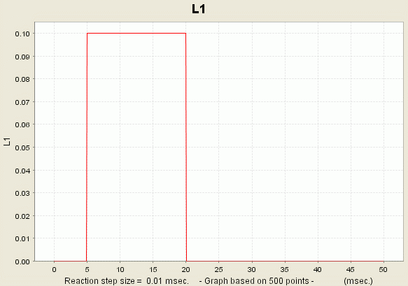
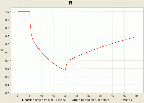
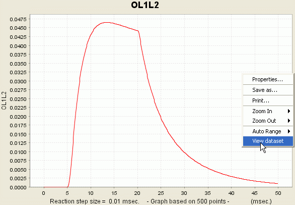
You can access the data if you right-click the plot and select the option 'View Dataset'.